Blog

The Gencove Team - Jul 16, 2024

Genomic prediction in maize using the Genomes to Fields (G2F) data and Gencove Explorer

Introduction

In this notebook we will demonstrate how to use Gencove Explorer to perform genomic prediction in maize.

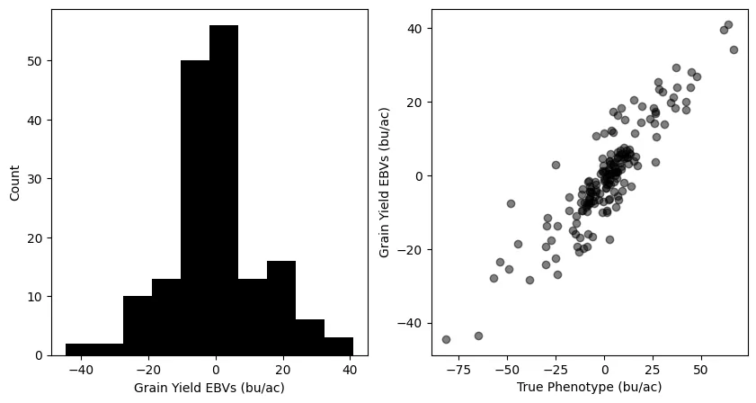
Specifically, we will be building a genomic prediction model for maize grain yield. Genomic prediction is a technique from statistical genetics that uses genome-wide genetic markers to estimate the breeding value (sometimes referred to as genetic merit) of plants or animals in modern breeding programs. This estimated breeding value (EBV) can be used to identify and selectively breed the best individuals in the population in order to improve the agronomically relevant traits.

Genomic prediction has revolutionized breeding programs across various agricultural species due to its cost-effectiveness and accuracy. Genomic prediction often approaches the accuracy of direct phenotyping but at a fraction of the cost. Additionally, it enables the estimation of breeding values for traits not directly expressed by an individual, such as a dairy bull's genetic potential for milk quality traits in his female offspring. For an in-depth understanding of the goals and foundational theory of genomic prediction, see the original work in the field by Meuwissen et al.

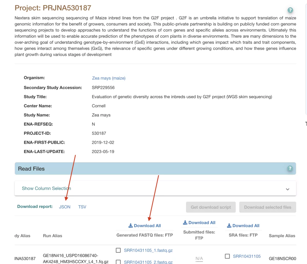
Here we will be using GenomesToFields (G2F) maize phenotype data here, and corresponding low-pass whole genome sequence data (approx 1-3x genomic coverage per line) from NCBI Project PRJNA530187.

The following code will be executed on a Gencove Explorer instance; through the use of the Gencove Explorer SDK, we will submit a high compute job to the analysis cluster that accompanies each Explorer deployment for data retrieval and processing, before downloading the results to our local instance in order to perform further analysis.

At a high level, we will perform the following steps:

Retrieve and clean the G2F maize phenotype data (grain yields).
Download low-pass whole genome sequence data from NCBI SRA for the same maize lines.
Upload the sequence data to the Gencove SaaS for imputation.
Prepare and clean the resulting imputed genotypes for genomic prediction.
Fit a Genomic Best Linear Unbiased Prediction (GBLUP) model using GEMMA on the Explorer analysis cluster
Explore and visualize the results
Upload the results to Explorer cloud storage.

Data Retrieval

First, we retrieve the genotype and phenotype data associated with the G2F project:

We manually download the g2f_2018_hybrid_data_clean.csv file from the G2F phenotype data records and store it locally. This data includes grain yield estimates from multiple maize hybrids across several growing locations. We will process this hybrid data to extract grain yield phenotype estimates for each female maize inbred line used to make the hybrid cross.
We download raw FASTQ sequence data from NCBI SRA to local storage. We will upload this data later to the Gencove SaaS for imputation. There are many ways to retreive sequence data from the SRA, I find it easiest to navigate to the project on ENA and download their Download All script for the FASTQ files associated with the project. This should download a shell script called ena-file-download-read_run-PRJNA530187-fastq_ftp-*DATE*.sh, where *DATE* contains the date it was downloaded. This shell script contains POSIX code for downloading the FASTQ files from this project. See screenshot below for Download All link (see right arrow). While at this site, also download the JSON report (see left arrow below), we will use this file to convert SRA names to inbred line names later.

Phenotype data processing

The phenotype data is from hybrid maize F1s. We want the estimate of the grain yield value of the female line (all hybrid IDs in this data set are given as {female_parent_ID}/{male_parent_ID}), while controlling for the effects of location and the male parent. We will do this by processing the data to build an appropriate data set, and then fitting a linear model and extracting the female inbred line coefficient estimates for the grain yield phenotype.

In [1]:

# Install pip dependencies
!pip install statsmodels pandas

import json, random
import pandas as pd
import statsmodels.formula.api as smf

# read hybrid data into pandas and unnest the hybrid pedigree into female and male tester lines
dat_tmp = pd.read_csv("g2f_2018_hybrid_data_clean.csv")
fem = [i.split("/")[0] for i in dat_tmp.Pedigree]
tester = [i.split("/")[1] if "/" in i else "" for i in dat_tmp.Pedigree]

# make simplified dataframe, that includes our grain yield phenotype, female and male (tester) lines, and field location
dat = pd.DataFrame(
    {
        "yld": dat_tmp["Grain Yield [bu/A]"],
        "fem": fem,
        "tester": tester,
        "loc": dat_tmp["Field-Location"],
    }
)

# fit a regression and extract grain yld coef for female inbred
results = smf.ols("yld ~ loc + fem + tester", data=dat).fit()
yld_coeff = {
    i[0].replace("fem[T.", "").replace("]", ""): i[1]
    for i in results.params.items()
    if i[0].startswith("fem")
}  # isolate coefficients for "fem", the female inbred

# have a look at a few estimates
print(list(yld_coeff.items())[:5])

Out [1]:

[('2369', 7.81621437730225), ('9855HR', 40.841023907156064), ('B14A', -51.69482967028079), ('B37', -25.906411184529315), ('B73', 11.857246244237821)]

That gives us our prediction of grain yield by female inbred line, stored as a python dictionary called yld_coeff. Next we need to download public low-pass sequence data for these same lines and impute it using the Gencove SaaS.

Genotype data wrangling and imputation on Gencove SaaS

This work involves two steps; first, we parse the JSON file we downloaded from ENA to associate NCBI-SRA IDs with the corresponding inbred lines names we extracted grain yield estimates from above.

Then, to streamline this demonstration, we randomly select 200 lines from the 535 available to download.

In [2]:

with open("filereport_read_run_PRJNA530187_json.txt", "r") as f:
    seq_dat = json.load(f)

ok_srr = []
srr2name = {}
for i in seq_dat:
    srr = i["run_accession"]
    name = i["sample_title"]
    if name in yld_coeff:
        ok_srr.append(srr)
        srr2name[srr] = name
print(
    len(set(ok_srr))
)  # 535 total we can download, so now edit the download script to only get those accessions

# we will select 200 for our future work
random.seed(43)  # make reproducible
fin_srr = random.sample(ok_srr, 200)
print(len(set(fin_srr)))

# and now modify the ENA shell script to download only those 200 indv
sh_out = []
for cmd in open("ena-file-download-read_run-PRJNA530187-fastq_ftp-20240402-2057.sh"):
    for j in fin_srr:
        if j in cmd:
            sh_out.append(cmd)

print(len(sh_out))  # 400 files, b/c paired end reads

# write out new shell script and run
with open("ena.mod.download.sh", "w") as shell:
    for i in sh_out:
        shell.write(i)

Out [2]:

535
200
400

We then download the data to our local Explorer instance using the generated shell script.

In [3]:

!chmod 755 ena.mod.download.sh
!./ena.mod.download.sh

Out [3]:

--2024-04-03 22:55:00--  ftp://ftp.sra.ebi.ac.uk/vol1/fastq/SRR104/033/SRR10431533/SRR10431533_1.fastq.gz
           => ‘SRR10431533_1.fastq.gz’
Resolving ftp.sra.ebi.ac.uk (ftp.sra.ebi.ac.uk)... 193.62.193.165
Connecting to ftp.sra.ebi.ac.uk (ftp.sra.ebi.ac.uk)|193.62.193.165|:21... connected.
Logging in as anonymous ... Logged in!
==> SYST ... done.    ==> PWD ... done.
==> TYPE I ... done.  ==> CWD (1) /vol1/fastq/SRR104/033/SRR10431533 ... done.
==> SIZE SRR10431533_1.fastq.gz ... 1676842370
==> PASV ... done.    ==> RETR SRR10431533_1.fastq.gz ... done.
Length: 1676842370 (1.6G) (unauthoritative)

SRR10431533_1.fastq 100%[===================>]   1.56G  36.5MB/s    in 45s  
...

We now have 400 FASTQs downloaded locally. Next we will change the NCBI-SRA FASTQ file names to the sample names from the G2F data, and make some small tweaks to remove underscores so they match the file name convetions of the Gencove pipeline.

In [4]:

import glob, os, re

# now extract line names and rename our downloaded FASTQs so that they have the line name.
# For the Gencove SaaS we are going to change all underscores in the file name to dashes
# and replace _1 or _2 with _R1 or _R2.
# see file naming conventions here https://docs.gencove.com/main/the-gencove-cli/#file-naming-convention

pattern = r"([12])(\.fastq\.gz)"  # regex pattern to fix R1/R2 names
replacement = r"R\1\2"
for i in seq_dat:
    srrname = i["run_accession"]
    linename = i["sample_title"]
    g = glob.glob(f"{srrname}*")
    for f in g:
        f1 = f.replace(
            srrname, linename.replace("_", "-")
        )  # replace underscore from line name and swap with srr
        f2 = re.sub(pattern, replacement, f1)
        os.rename(f, f2)  # rename all files

In [5]:

# first make a dir called reads and move the FASTQ files to it
!mkdir reads
!mv *fastq.gz reads
!ls reads/ | wc -l  # 342 FASTQs

Out [5]:

After renaming, it appears we have less than 400 FASTQs. It turns out this is because there are multiple NCBI-SRA IDs associated with the same inbred line in the G2F data. In renaming files we have overwritten one with another. So instead of using 200 lines for genomic prediction we will use the 171 unique lines we have. In a real project we'd go back and combine the NCBI-SRA FASTQs into a single file.

However, both 171 and 200 individuals are quite small samples sizes for genomic prediction, but fine for our purposes of demonstrating how to build a genomic prediction model, so we will proceed with 171 individuals.

Upload to Gencove SaaS and impute

The samples we downloaded appear to be 1-3x genomic coverage, which is somewhat low for direct variant calling, so instead we will use imputation. To accomplish this we will run these samples through the Gencove MAIZE LOW-PASS V1.2 imputation pipeline, which imputes whole genome low-pass sequence data to approx 86 million variant sites. I have already created a project in my account and I will supply the Gencove CLI upload command with my run project ID so my fastq samples will begin imputation immediately. The samples will be imputed in parallel in the cloud in a few hours.

In [6]:

!gencove upload reads --run-project-id b57e0aad-e443-47f8-943f-c1cd0c853221

Out [6]:

WARNING: The Gencove upload area is a temporary storage. Log into the dashboard and assign uploaded files to a project in order to avoid automatic deletion.
Files will be uploaded to: gncv://cli-20240404174359-10e2cc0dd89141e18ef7cf7c4393b2a2
Checking if file was already uploaded: Mo44-PHW65-0011_R1.fastq.gz
Uploading reads/Mo44-PHW65-0011_R1.fastq.gz to gncv://cli-20240404174359-10e2cc0dd89141e18ef7cf7c4393b2a2/Mo44-PHW65-0011_R1.fastq.gz
Uploading: 100% [############] Time:  0:00:17 Elapsed Time: 0:00:17  77.8 MiB/s
...

After a few hours, the pipeline has completed for these samples, and we generate a merged VCF file for these 171 lines using the Gencove CLI.

In [7]:

!gencove projects create-merged-vcf b57e0aad-e443-47f8-943f-c1cd0c853221

Out [7]:

Issued merge request for project b57e0aad-e443-47f8-943f-c1cd0c853221
f979d726-57c1-411b-a0d4-24e38a4975d3	2024-04-05T15:24:52.135057+00:00	received

Prepare genotype data for genomic prediction

We can now use the Explorer SDK to download the merged VCF and begin preparation of the genotype and phenotype data so we can train a genomic prediction model.

In [8]:

from gencove_explorer import get_projects

p = get_projects("b57e0aad-e443-47f8-943f-c1cd0c853221", file_types=["impute-vcf-merged"])
merged_vcf = p[0].files["impute-vcf-merged"]
merged_vcf.download()

Out [8]

Downloading: 100%|##########| 39.7G/39.7G [12:07<00:00, 54.6MB/s]
...

Installing necessary packages

We will use plink to extract sites and GEMMA to run GBLUP genomic prediction, so we must install them:

In [9]:

# plink1.9 and 2
!wget https://s3.amazonaws.com/plink1-assets/plink_linux_x86_64_20231211.zip
!unzip plink_linux_x86_64_20231211.zip
!wget https://s3.amazonaws.com/plink2-assets/alpha5/plink2_linux_x86_64_20240105.zip
!unzip plink2_linux_x86_64_20240105.zip 

# gemma
!wget https://github.com/genetics-statistics/GEMMA/releases/download/v0.98.5/gemma-0.98.5-linux-static-AMD64.gz
!gunzip gemma-0.98.5-linux-static-AMD64.gz 
!mv gemma-0.98.5-linux-static-AMD64 gemma
!chmod 755 gemma

Out [9]:

--2024-04-06 00:05:32--  https://s3.amazonaws.com/plink1-assets/plink_linux_x86_64_20231211.zip
Resolving s3.amazonaws.com (s3.amazonaws.com)... 54.231.201.216, 54.231.204.104, 52.217.173.96, ...
Connecting to s3.amazonaws.com (s3.amazonaws.com)|54.231.201.216|:443... connected.
...

Extract high MAF sites and downsample to 100k sites

The VCF contains 171 lines and over 86.5M variants. For simplicity, we will downsample the vcf to 100k sites high-frequency sites (MAF >10%), and also remove multiallelic sites.

In [10]:

# find high MAF sites and make filtered vcf with only those sites
!bcftools index {merged_vcf.local}

# norm and exclude multallelics for simplicty
!bcftools norm -m +any {merged_vcf.local} --threads 4 | bcftools view -m2 -M2 --threads 4 -Oz -o normed.biallelic.merged.vcf.gz

# extract high MAF sites
!./plink --vcf normed.biallelic.merged.vcf.gz --maf 0.10 --recode vcf --out high.maf
!cat high.maf.vcf | cut -f 1,2 | shuf -n 100000 > 100k.sites

# generate the filtered vcf with only the 100k high-frequency sites
!bcftools view -T 100k.sites high.maf.vcf -Oz -o filtered.100k.vcf.gz

Prep the VCF and phenotype data for GEMMA

We will output our female grain yield estimates sorted in yld_coeff in a format that plink2 can read, all while making sure the phenotype records are kept in the same order as the genotype records. The final plink2 command creates .bed, .bim, and .fam files (with the grain_yld_mod prefix), that GEMMA can read. This concludes our data wrangling.

In [11]:

line_order = !bcftools query -l filtered.100k.vcf.gz  # get order of indv in vcf
plink_pheno_file = open("plink.pheno.txt", "w")

# reformat line names
for i in line_order:
    indv = i.split("_")[0].replace(
        "-", "_"
    )
    yld_val = yld_coeff[indv]
    print(0, i, yld_val, file=plink_pheno_file, sep="\t")
plink_pheno_file.close()

!./plink2 --vcf filtered.100k.vcf.gz --make-bed --pheno plink.pheno.txt --out grain_yld_mod

Out [11]:

PLINK v2.00a5.10LM 64-bit Intel (5 Jan 2024)   www.cog-genomics.org/plink/2.0/
(C) 2005-2024 Shaun Purcell, Christopher Chang   GNU General Public License v3
Logging to grain_yld_mod.log.
Options in effect:
  --make-bed
  --out grain_yld_mod
  --pheno plink.pheno.txt
  --vcf filtered.100k.vcf.gz

Start time: Wed May  8 18:23:46 2024
31548 MiB RAM detected, ~26018 available; reserving 15774 MiB for main
workspace.
Using up to 8 compute threads.
--vcf: 99999 variants scanned.
--vcf: grain_yld_mod-temporary.pgen + grain_yld_mod-temporary.pvar.zst +
grain_yld_mod-temporary.psam written.
171 samples (0 females, 0 males, 171 ambiguous; 171 founders) loaded from
grain_yld_mod-temporary.psam.
99999 variants loaded from grain_yld_mod-temporary.pvar.zst.
1 quantitative phenotype loaded (171 values).
Writing grain_yld_mod.fam ... done.
Writing grain_yld_mod.bim ... done.
Writing grain_yld_mod.bed ... done.
End time: Wed May  8 18:23:46 2024

Genomic prediction modeling

Now that we've got a complete plink dataset with which to work, we can start on the genomic prediction analysis. We will first estimate the marker h² using GEMMA, and then fit a GBLUP model and estimate its accuracy using 5-fold cross-validation.

Take a look at the marker h² with GEMMA.

A good place to start with genomic prediction is to determine the marker h². This is the proportion of the total phenotypic variance that can be explained by genotype differences between our individuals. To estimate marker h² with GEMMA, we first need extract a genetic relationship matrix (GRM; -gk 1 flag in GEMMA) and use that to fit a univariate mixed effects linear model to the data. The latter model reports an estimate of the h² (given as pve estimate, AKA the proportion of phenotypic variance explained by the genotypic data).

In [12]:

!./gemma -bfile grain_yld_mod -gk 1 -o grm #make the GRM
!./gemma -bfile grain_yld_mod -lmm 3 -k output/grm.cXX.txt -o yield_h2

Out [12]:

GEMMA 0.98.5 (2021-08-25) by Xiang Zhou, Pjotr Prins and team (C) 2012-2021
Reading Files ... 
## number of total individuals = 171
## number of analyzed individuals = 171
## number of covariates = 1
## number of phenotypes = 1
## number of total SNPs/var        =    99999
## number of analyzed SNPs         =    99999
Calculating Relatedness Matrix ... 
================================================== 100%
**** INFO: Done.
GEMMA 0.98.5 (2021-08-25) by Xiang Zhou, Pjotr Prins and team (C) 2012-2021
Reading Files ... 
## number of total individuals = 171
## number of analyzed individuals = 171
## number of covariates = 1
## number of phenotypes = 1
## number of total SNPs/var        =    99999
## number of analyzed SNPs         =    99999
Start Eigen-Decomposition...
pve estimate =0.524341
se(pve) =0.124963
================================================== 100%
**** INFO: Done.

As indicated above, the h² is ~0.52. This h² suggests that there is genetic variation that can be captured as marker effects and can be used to predict EBVs for grain yield. The standard error (se(pve)) is ~0.125, which is quite large, but this is expected due to our small sample size for genomic prediction.

Fit a GBLUP model and evaluate its accuracy using 5-fold cross-validation

The GBLUP uses the genetic covariance between individuals (in our case, estimated using our 100k marker genotype data), plus the phenotype values (in our case the grain yield coefficients), to fit a mixed effects model to the data and extract EBVs. A thorough description of the GBLUP method can be found here. Importantly, the GBLUP applies shrinkage to the EBVs, such that each individuals EBV is pulled toward the population grand mean, making the EBVs provably more robust.

In GEMMA, the GBLUP is fitted using the -bslmm 2 flag. We will perform 5-fold cross-validation by masking out 1/5th of the lines and fitting the GBLUP on the remainder and repeating 5 times. When finished, we will compare the predicted EBVs of the masked lines to the "true" phenotypic values as estimated above.

It is customary to compare the EBVs to the true phenotypes using Pearson's correlation coefficient (r), and in this framework we expect r to approach the predicted h² above.

Before we begin, we will make a copy of our phenotype records (.fam file), so that we can make substitute copies with NA masking out phenotype records.

In [13]:

!cp grain_yld_mod.fam orig.grain_yld_mod.fam # save original fam file

Next, we proceed with the 5-fold cross-validation, a critical step in validating the robustness of our genomic prediction model. Given the computational demands of this step, it is beneficial to parallelize the process. We will utilize the powerful features offered by the Gencove Explorer SDK, specifically the Analysis and File classes. These classes facilitate efficient and scalable cloud-based computation, allowing for streamlined execution and management of parallel compute tasks directly from an Explorer notebook.

We begin by importing necessary objects from the gencove_explorer SDK. The File object is used to handle file operations seamlessly between local and remote (cloud) storage. Files such as the genotype and phenotype datasets (fam, bed, bim) and the executable for the GEMMA software are encapsulated within File objects. These objects are then uploaded to the cloud, ensuring that all necessary data is available in the cloud environment where the computation will occur.

The work function encapsulates the core logic for running a single fold of the cross-validation. It is designed to be executed in parallel across multiple cloud nodes, each handling a different subset of the data (one fold). Within this function, the following key operations occur:

File Downloading: Each node downloads its required input files from the cloud, ensuring that the latest and correct versions of the files are used. This includes the fam, bed, bim files, and the GEMMA executable.

Data Masking: To perform the cross-validation, phenotypic values (fam file) for the test set are masked (set to NA). This ensures that the model cannot use these values during training, mimicking a scenario where these values are unknown and need to be predicted.

Model Fitting and Prediction: The GEMMA software is used to fit a genomic best linear unbiased prediction (GBLUP) model using the masked dataset and subsequently to predict the masked phenotypic values.

Results Handling: The true phenotypic values and the predicted values are extracted, and the results are stored back in the AnalysisContext object, making them accessible for further analysis or aggregation across all folds.

In [14]:

from gencove_explorer.models import File
from gencove_explorer.analysis import Analysis, AnalysisContext

random.seed(15)  # make repeatable
test_sets = [
    random.choice([0, 1, 2, 3, 4])
    for i in range(len(list(open("orig.grain_yld_mod.fam"))))
]  # randomly assign each line to 1 test set

fam_file = File(local="orig.grain_yld_mod.fam", remote="orig.grain_yld_mod.fam")
bed_file = File(local="grain_yld_mod.bed", remote="grain_yld_mod.bed")
bim_file = File(local="grain_yld_mod.bim", remote="grain_yld_mod.bim")
gemma_exe = File(local="gemma", remote="gemma")
for i in [fam_file, bed_file, bim_file, gemma_exe]:
    i.upload(force=True)  # upload each to cloud storage

# Work function that will be run on the cluster
def work(ac: AnalysisContext):
    """
    Run GBLUP calculation on one test set. this function will be run in parallel
    on a cloud cluster on each test set
    
    Args:
        ac (AnalysisContext): the analysis context object that contains the input
        files and test set info
    
    Returns:
        None, the results will be stored in the analysis context object as `results`

    """
    fam_file_obj = (
        ac.input_shared.fam_file.download()
    )  # get the shared fam file from the analysis context
    bed_file_obj = (
        ac.input_shared.bed_file.download()
    )  # get the shared bed file from the analysis context
    bim_file_obj = (
        ac.input_shared.bim_file.download()
    )  # get the shared bim file from the analysis context
    gemma_exe_obj = (
        ac.input_shared.gemma_exe.download()
    )  # get the shared gemma exe from the analysis context
    !cp {bed_file_obj.local} grain_yld_mod.bed
    !cp {bim_file_obj.local} grain_yld_mod.bim
    !cp {gemma_exe_obj.local} gemma
    !chmod 755 gemma

    test_num = ac.input[0]  # get the shared test num from the analysis context
    test_sets = ac.input[1]  # get the shared test set from the analysis context

    fam_file = [i.strip().split() for i in open(fam_file_obj.local)]
    
    with open("grain_yld_mod.fam", "w") as masked_fam:
        for t, v in zip(test_sets, fam_file):
            if t == test_num:
                v[-1] = "NA"  # test pheno to NA if line is in this test set
            masked_fam.write("\t".join(v) + "\n")

    # fit with test set to NA
    !./gemma -bfile grain_yld_mod -bslmm 2 -o gblup  # bslmm 2 is the GBLUP
    
    # predict test
    !./gemma -bfile grain_yld_mod -predict 1 -epm output/gblup.param.txt -o predict
    
    fam_file = [i.strip().split() for i in open(fam_file_obj.local)]  # fresh copy of fam file
    true_pheno = [float(v[-1]) for t, v in zip(test_sets, fam_file) if t == test_num]
    pred_pheno = [float(i) for i in open("output/predict.prdt.txt") if "NA" not in i]
    ac.output.results = [(true_pheno, pred_pheno)]

Now we use the InputShared object to store shared inputs our work function will need and the JobDefinition to specify our compute resource needs for each job.

Then we create an Analysis object called an and submit our 5 jobs.

In [15]:

from gencove_explorer.analysis import InputShared, JobDefinition

input_shared = InputShared(
    fam_file=fam_file, bed_file=bed_file, bim_file=bim_file, gemma_exe=gemma_exe
)  # define the shared input files

job_defn = JobDefinition(cpu=2, memory_mb=8192, storage_gb=50)  # define the compute resources needed for the job

# analysis fucntion
an = Analysis(
    function=work,
    input=[(test_num, test_sets) for test_num in range(5)],  # each of the 5 inputs contains the test set number and the list of assigned test set for each indv
    job_definition=job_defn,
    input_shared=input_shared,
)

an.run()  # submit the analysis to the cloud cluster

▰▱▱▱▱▱▱ Submitting remote job✅ Remote job submitted

Out [15]:

Analysis(input=[(0, [1, 0, 4, 0, 1, 1, 0, 0, 1, 2, 1, 0, 2, 3, 2, 2, 3, 2, 2, 1, 1, 2, 2, 1, 2, 4, 3, 1, 4, 3, 3, 3, 0, 3, 4, 2, 3, 4, 2, 3, 3, 0, 3, 0, 1, 1, 4, 1, 4, 0, 2, 4, 3, 1, 0, 0, 3, 0, 0, 3, 4, 2, 3, 4, 1, 1, 4, 4, 2, 0, 1, 2, 2, 1, 2, 3, 3, 2, 3, 0, 2, 3, 1, 0, 3, 3, 3, 0, 2, 0, 2, 0, 0, 3, 0, 2, 1, 3, 4, 3, 3, 0, 4, 0, 3, 0, 4, 3, 1, 4, 3, 2, 0, 4, 0, 0, 2, 3, 3, 2, 0, 4, 2, 4, 3, 2, 4, 0, 3, 3, 0, 2, 4, 3, 4, 0, 1, 2, 1, 3, 4, 2, 2, 1, 4, 2, 3, 2, 0, 4, 2, 1, 2, 0, 1, 4, 0, 4, 3, 2, 1, 2, 0, 2, 2, 3, 4, 4, 4, 3, 4]), (1, [1, 0, 4, 0, 1, 1, 0, 0, 1, 2, 1, 0, 2, 3, 2, 2, 3, 2, 2, 1, 1, 2, 2, 1, 2, 4, 3, 1, 4, 3, 3, 3, 0, 3, 4, 2, 3, 4, 2, 3, 3, 0, 3, 0, 1, 1, 4, 1, 4, 0, 2, 4, 3, 1, 0, 0, 3, 0, 0, 3, 4, 2, 3, 4, 1, 1, 4, 4, 2, 0, 1, 2, 2, 1, 2, 3, 3, 2, 3, 0, 2, 3, 1, 0, 3, 3, 3, 0, 2, 0, 2, 0, 0, 3, 0, 2, 1, 3, 4, 3, 3, 0, 4, 0, 3, 0, 4, 3, 1, 4, 3, 2, 0, 4, 0, 0, 2, 3, 3, 2, 0, 4, 2, 4, 3, 2, 4, 0, 3, 3, 0, 2, 4, 3, 4, 0, 1, 2, 1, 3, 4, 2, 2, 1, 4, 2, 3, 2, 0, 4, 2, 1, 2, 0, 1, 4, 0, 4, 3, 2, 1, 2, 0, 2, 2, 3, 4, 4, 4, 3, 4]), (2, [1, 0, 4, 0, 1, 1, 0, 0, 1, 2, 1, 0, 2, 3, 2, 2, 3, 2, 2, 1, 1, 2, 2, 1, 2, 4, 3, 1, 4, 3, 3, 3, 0, 3, 4, 2, 3, 4, 2, 3, 3, 0, 3, 0, 1, 1, 4, 1, 4, 0, 2, 4, 3, 1, 0, 0, 3, 0, 0, 3, 4, 2, 3, 4, 1, 1, 4, 4, 2, 0, 1, 2, 2, 1, 2, 3, 3, 2, 3, 0, 2, 3, 1, 0, 3, 3, 3, 0, 2, 0, 2, 0, 0, 3, 0, 2, 1, 3, 4, 3, 3, 0, 4, 0, 3, 0, 4, 3, 1, 4, 3, 2, 0, 4, 0, 0, 2, 3, 3, 2, 0, 4, 2, 4, 3, 2, 4, 0, 3, 3, 0, 2, 4, 3, 4, 0, 1, 2, 1, 3, 4, 2, 2, 1, 4, 2, 3, 2, 0, 4, 2, 1, 2, 0, 1, 4, 0, 4, 3, 2, 1, 2, 0, 2, 2, 3, 4, 4, 4, 3, 4]), (3, [1, 0, 4, 0, 1, 1, 0, 0, 1, 2, 1, 0, 2, 3, 2, 2, 3, 2, 2, 1, 1, 2, 2, 1, 2, 4, 3, 1, 4, 3, 3, 3, 0, 3, 4, 2, 3, 4, 2, 3, 3, 0, 3, 0, 1, 1, 4, 1, 4, 0, 2, 4, 3, 1, 0, 0, 3, 0, 0, 3, 4, 2, 3, 4, 1, 1, 4, 4, 2, 0, 1, 2, 2, 1, 2, 3, 3, 2, 3, 0, 2, 3, 1, 0, 3, 3, 3, 0, 2, 0, 2, 0, 0, 3, 0, 2, 1, 3, 4, 3, 3, 0, 4, 0, 3, 0, 4, 3, 1, 4, 3, 2, 0, 4, 0, 0, 2, 3, 3, 2, 0, 4, 2, 4, 3, 2, 4, 0, 3, 3, 0, 2, 4, 3, 4, 0, 1, 2, 1, 3, 4, 2, 2, 1, 4, 2, 3, 2, 0, 4, 2, 1, 2, 0, 1, 4, 0, 4, 3, 2, 1, 2, 0, 2, 2, 3, 4, 4, 4, 3, 4]), (4, [1, 0, 4, 0, 1, 1, 0, 0, 1, 2, 1, 0, 2, 3, 2, 2, 3, 2, 2, 1, 1, 2, 2, 1, 2, 4, 3, 1, 4, 3, 3, 3, 0, 3, 4, 2, 3, 4, 2, 3, 3, 0, 3, 0, 1, 1, 4, 1, 4, 0, 2, 4, 3, 1, 0, 0, 3, 0, 0, 3, 4, 2, 3, 4, 1, 1, 4, 4, 2, 0, 1, 2, 2, 1, 2, 3, 3, 2, 3, 0, 2, 3, 1, 0, 3, 3, 3, 0, 2, 0, 2, 0, 0, 3, 0, 2, 1, 3, 4, 3, 3, 0, 4, 0, 3, 0, 4, 3, 1, 4, 3, 2, 0, 4, 0, 0, 2, 3, 3, 2, 0, 4, 2, 4, 3, 2, 4, 0, 3, 3, 0, 2, 4, 3, 4, 0, 1, 2, 1, 3, 4, 2, 2, 1, 4, 2, 3, 2, 0, 4, 2, 1, 2, 0, 1, 4, 0, 4, 3, 2, 1, 2, 0, 2, 2, 3, 4, 4, 4, 3, 4])], function=work, input_shared=InputShared(fam_file=File(local=PosixPath('orig.grain_yld_mod.fam'), remote=NamedFile(path='orig.grain_yld_mod.fam')), bed_file=File(local=PosixPath('grain_yld_mod.bed'), remote=NamedFile(path='grain_yld_mod.bed')), bim_file=File(local=PosixPath('grain_yld_mod.bim'), remote=NamedFile(path='grain_yld_mod.bim')), gemma_exe=File(local=PosixPath('gemma'), remote=NamedFile(path='gemma'))), job_definition=JobDefinition(cpu=2, memory_mb=8192, storage_gb=50, attempts=1, image=Image(name='362435828402.dkr.ecr.us-east-1.amazonaws.com/explorer-dev-batch'), timeout_seconds=3600, privileged=False), id='2024-05-08T202258_work_45e343c03091495281628105ae4432c5', name=None, pip_packages=[], conda_packages=[])

We can use the an.status() method to check on the status of the jobs we submitted. Once all 5 have finished, the output will look as it does below.

In [17]:

an.status()

Out [17]:

{
    "status": "SUCCEEDED",
    "status_reason": None,
    "child_jobs": 5,
    "status_summary": {
        "STARTING": 0,
        "FAILED": 0,
        "RUNNING": 0,
        "SUCCEEDED": 5,
        "RUNNABLE": 0,
        "SUBMITTED": 0,
        "PENDING": 0,
    },
}

Now with the 5 cross-validation cloud jobs complete, we can retrieve our results using the get_output method from the an Analysis object and compute the 5-fold cross-validation accuracy.

In [19]:

import numpy as np

def cor(a, b):
    return np.corrcoef(a, b)[0][1]

corrs_true, corrs_ebv = [], []
for idx in range(5):
    true_pheno, pred_pheno = an.get_output(job_index=idx).results[0]  # stored as `results` in our work function
    corrs_true.extend(true_pheno)
    corrs_ebv.extend(pred_pheno)

print("Mean 5-fold cross-validation Pearsons correlation:", cor(corrs_true, corrs_ebv))

Out [19]:

Mean 5-fold cross-validation Pearsons correlation: 0.5142680003789858

Cross-validated Results

5-fold cross-validation resulted in an average prediction accuracy of about 51.4% as measured by Pearson's correlation. This gives us an estimate of the performance of our GBLUP method for producing EBVs on out-of-sample maize inbred lines. Thus, if we applied this genomic prediction model to other individuals from the same population, we'd expect to be able to predict ~51.4% of the total phenotypic variance using these 100K genotypic markers.

Fitting the full GBLUP model

Next we want to extract the marker effects. These are the variant specific weights for each of our 100K sites. For the full GBLUP model, we simply fit GEMMA -bslmm 2 without masking any individual's phenotype.

In [20]:

!cp orig.grain_yld_mod.fam grain_yld_mod.fam
!./gemma -bfile grain_yld_mod -bslmm 2 -o final.gblup

Out [20]:

GEMMA 0.98.5 (2021-08-25) by Xiang Zhou, Pjotr Prins and team (C) 2012-2021
Reading Files ... 
## number of total individuals = 171
## number of analyzed individuals = 171
## number of covariates = 1
## number of phenotypes = 1
## number of total SNPs/var        =    99999
## number of analyzed SNPs         =    99999
Start Eigen-Decomposition...
pve estimate =0.524341
se(pve) =0.124963
Calculating UtX...
**** INFO: Done.

Explore the results

First, the final marker effects are below (given as alpha). These marker effects can be used to estimate EBVs on other female maize inbreds genotyped at the same 100k markers.

In [21]:

!head output/final.gblup.param.txt

Out [21]:

chr	rs	ps	n_miss	alpha	beta	gamma
1	1-458678	503641	0	7.532010e-04	0.000000e+00	0.000000e+00
1	1-505559	550518	0	-1.770978e-03	0.000000e+00	0.000000e+00
1	1-510158	555117	0	1.538598e-03	0.000000e+00	0.000000e+00
1	1-643432	687668	0	2.909762e-03	0.000000e+00	0.000000e+00
1	1-806151	838168	0	2.157416e-03	0.000000e+00	0.000000e+00
1	1-806624	838641	0	1.809730e-03	0.000000e+00	0.000000e+00
1	1-839922	871938	0	8.885294e-04	0.000000e+00	0.000000e+00
1	1-858673	890689	0	1.681004e-03	0.000000e+00	0.000000e+00
1	1-884825	916842	0	-1.916306e-03	0.000000e+00	0.000000e+00

And we can plot a histogram of the EBVs and a scatter plot of the observed phenotypes vs. the GBLUP estimates.

In [22]:

from matplotlib import pyplot as plt

plt.rcParams["figure.figsize"] = [10, 5]

ebvs = [float(i.strip()) for i in open("output/final.gblup.bv.txt")]
truth = [float(i.strip().split()[-1]) for i in open("orig.grain_yld_mod.fam")]
plt.subplot(121)
plt.hist(ebvs, color="k")
plt.xlabel("Grain Yield EBVs (bu/ac)")
plt.ylabel("Count")

plt.subplot(122)
plt.scatter(truth, ebvs, color="k", alpha=0.5)
plt.xlabel("True Phenotype (bu/ac)")
plt.ylabel("Grain Yield EBVs (bu/ac)")

Out [22]:

Text(0, 0.5, 'Grain Yield EBVs (bu/ac)')

As you can see above, the grain yield EBVs are centered on zero and are in the same units as the phenotype (bushels per acre in this case). An inbred line with an EBV of zero is expected to have a genetic merit equivalent to the population grand mean. Individuals on the positive end of the EBV scale are expected to transmit genetic performance greater than the population mean, and the reciprocal for negative EBVs. Using these EBVs we can make selection decisions in a breeding program, and advance only individuals with the most beneficial EBVs.

Moreover, EBVs are additive, meaning if we cross and invidual with a grain yield EBV of +10 with another individual with an EBV of +20, we expect their average offspring to be the midparent EBV, which is +15.

Finally, we will use the Gencove Explorer SDK to upload our GBLUP EBVs to shared cloud storage (at e://org) so we can easily share with colleagues.

In [23]:

!gencove explorer data cp output/final.gblup.bv.txt e://org/final.gblup.bv.txt

Out [23]:

upload: output/final.gblup.bv.txt to s3://gencove-explorer-e26d9b3e9db7/shared/files/final.gblup.bv.txt

Conclusion

Here we have demonstrated how to perform a genomic prediction analysis of a large dataset of whole-genome sequencing data by leveraging Gencove's base pipelines as well as Gencove Explorer and its associated SDK.

Using the Gencove platform in this notebook, we: (1) downloaded a large public maize data set, (2) cleaned the phenotype data, (3) imputed whole genome sequence using Gencove's automated pipelines, (3) fit a genomic prediction model for grain yield, (4) and validated its performance.

We illustrated the power of Gencove Explorer to manage and execute complex genomic analyses in a cloud environment, and how it can be used to streamline the process of heavy-duty computational tasks such as genomic prediction.

Get in touch with the Gencove team to start leveraging Explorer today >

UNLOCK the power of sequencing >